Numerical Settings
These are additional inputs that can be used to define the numerical approach and discretization. These inputs are largely intended for advanced research or testing purposes.
Number of Dimensions
Switch between two- and three-dimensional simulations. Warning: Three-dimensional simulations can be very computationally intensive. Kiva does not impose any limitations, but be warned: some three-dimensional simulations may require more memory than most computers have available.
| Required: | No |
| Type: | Integer |
| Constraints: | 2 or 3 |
| Default: | 2 |
Coordinate System
Allows the user to specify the coordinate system used for calculations. For Three-dimensional simulations, this must be CARTESIAN.
| Required: | No |
| Type: | Enumeration |
| Values: | CARTESIAN or CYLINDRICAL |
| Default: | CARTESIAN |
Two-Dimensional Approximation
These are methods of approximating three-dimensional foundation heat transfer using a two-dimensional coordinate system. Options are:
AP: Creates an infinite rectangle (Coordinate System =CARTESIAN) or a circle (Coordinate System =CYLINDRICAL) with the same area-to-perimeter ratio as the three-dimensional Polygon.RR: Creates the straight section (Coordinate System =CARTESIAN) or a rounded cap (Coordinate System =CYLINDRICAL) of a rounded rectangle with the same area and perimeter as the three-dimensional Polygon.BOUNDARY: Creates an infinite rectangle (Coordinate System =CARTESIAN) or a circle (Coordinate System =CYLINDRICAL) with an adjusted area-to-perimeter ratio from the three-dimensional Polygon. Adjustments are made to represent concave corners of the Polygon.CUSTOM: Creates an infinite rectangle (or parallel infinite rectangles) (Coordinate System =CARTESIAN) or a circle (or concentric circles) (Coordinate System =CYLINDRICAL) based on the specification of Length 1 and Length 2. This is an experimental feature where the three-dimensional Polygon is not used directly to define the approximation.
| Required: | No |
| Type: | Enumeration |
| Values: | AP, RR, BOUNDARY, or CUSTOM |
| Default: | BOUNDARY |
Length 1
Represents the outter width of an infinite rectangle (Coordinate System = CARTESIAN) or outer radius of a circle (Coordinate System = CYLINDRICAL).
| Required: | Depends |
| Type: | Numeric |
| Units: | m |
Length 2
Represents the inner width of parallel infinite rectangles (Coordinate System = CARTESIAN) or inner radius of concentric circles (Coordinate System = CYLINDRICAL).
| Required: | Depends |
| Type: | Numeric |
| Units: | m |
Use Symmetry
For three-dimensional simulations Kiva can detect planes of symmetry and automatically reduce the simulation domain by half (for a single plane of symmetry), or three quarters (for two planes of symmetry). If this is the case, then direction dependent boundary conditions such as incident solar and wind driven convection are averaged for the symmetric unit.
| Required: | No |
| Type: | Boolean |
| Default: | True |
Mesh
The mesh is a compound object that defines the refinement of cells within the calculation domain. Cells are defined within four distinct region types of the domain. The region bounding the foundation wall and insulation elements defines the near-field region. All other regions are defined either laterally (interior and far-field regions) or vertically (deep-field region) relative to the near-field region.
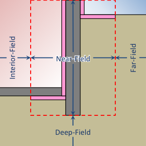
Illustration of regions (profile view)
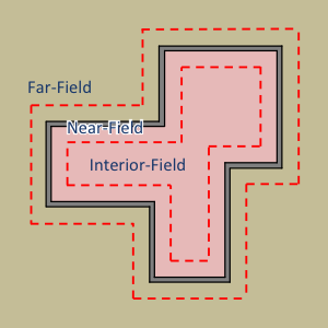
Illustration of regions (plan view)
Cells grow geometrically towards the far-field, deep-ground, and symmetry boundaries. Cells grow towards the center of each interior region and within each structural or insulation component. Example meshes are shown in the following figures.
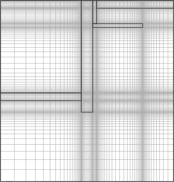
Profile view of a basement mesh
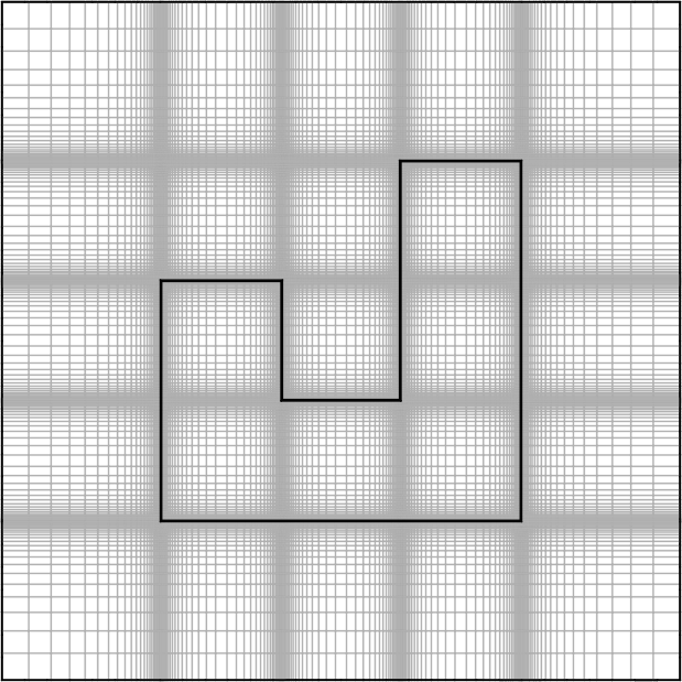
Plan view of a foundation mesh
Example:
Mesh:
  Minimum Cell Dimension: 0.02
  Maximum Near-Field Growth Coefficient: 1.5
  Maximum Deep-Field Growth Coefficient: 1.5
  Maximum Interior-Field Growth Coefficient: 1.5
  Maximum Far-Field Growth Coefficient: 1.5
| Required: | No |
| Type: | Compound object |
Minimum Cell Dimension
The minimum cell dimension defines the smallest possible dimension of a cell within the domain. This defines the allowable number of cells between element or region boundaries. The cells’ dimensions are allowed to increase to fit within a component or region boundaries according to the growth and distribution of the cells.
| Required: | No |
| Type: | Numeric |
| Units: | m |
| Default: | 0.02 |
Maximum Near-Field Growth Coefficient
The maximum size increase between neighboring cells within the near-field region.
| Required: | No |
| Type: | Numeric |
| Units: | dimensionless |
| Default: | 1.5 |
Maximum Deep-Field Growth Coefficient
The maximum size increase between neighboring cells within the deep-field region.
| Required: | No |
| Type: | Numeric |
| Units: | dimensionless |
| Default: | 1.5 |
Maximum Interior-Field Growth Coefficient
The maximum size increase between neighboring cells within the interior-field region.
| Required: | No |
| Type: | Numeric |
| Units: | dimensionless |
| Default: | 1.5 |
Maximum Far-Field Growth Coefficient
The maximum size increase between neighboring cells within the far-field region.
| Required: | No |
| Type: | Numeric |
| Units: | dimensionless |
| Default: | 1.5 |
Numerical Scheme
This defines the numerical scheme used for calculating domain temperatures for successive timesteps. Options are:
IMPLICIT, a fully implicit scheme with unconditional stability using an iterative solver,EXPLICIT, an explicit scheme with conditional stability,CRANK-NICOLSON, a partially implicit scheme with unconditional stability using an iterative solver (may exhibit oscillations),ADI, a scheme that solves each direction (X, Y, and Z) implicitly for equal sized sub-timesteps. The other two directions are solved explicitly. This allows for an exact solution of the linear system of equations without requiring an iterative solver. This scheme is extremely stable,ADE, a scheme that sweeps through the domain in multiple directions using known neighboring cell values. This scheme is very stable,STEADY-STATE, domain temperatures are calculated independently of previous timesteps using a steady-state solution from an iterative solver. This is often slower and less accurate than other methods.
| Required: | No |
| Type: | Enumeration |
| Values: | IMPLICIT, EXPLICIT, CRANK-NICOLSON, ADI, ADE, or STEADY-STATE |
| Default: | ADI |
f-ADI
When Numerical Scheme is ADI, this defines the weighting between the implicit, and explicit solutions in the sub-timesteps. In general, it is best to make this number very small.
| Required: | No |
| Type: | Numeric |
| Units: | dimensionless |
| Default: | 0.00001 |
Maximum Iterations
Maximum number of iterations allowed in search for a solution.
| Required: | No |
| Type: | Integer |
| Default: | 100000 |
Tolerance
Tolerance is defined as the relative \(\ell^2\)-norm of the residual when solving the linear system of equations.
| Required: | No |
| Type: | Numeric |
| Units: | Dimensionless |
| Default: | 1.0e-6 |